library(tidyverse)
library(tidymodels)
library(readxl)
library(openxlsx)
library(lubridate)
library(here)
library(devtools)
library(recipes)
library(rsample)
library(timetk)
library(glmnet)
library(tidyquant)
library(visdat)
library(janitor)
library(kableExtra)
library(caret)
library(rpart)
library(rpart.plot)
library(pdp)
library(vip)
library(GGally)
library(car)
library(ggcorrplot)
library(ggdensity)
library(tidyquant)
library(scico)
library(paletteer)
library(earth)
library(vip)
library(ranger)
library(h2o)
library(xgboost)
library(modeltime)
library(caret)
library(lares)
library(lmtest)
library(nortest)
library(auditor)
library(DALEXtra)
library(modelStudio)
library(patchwork)
What determines the price of houses in Bilbao? I want to investigate this question using Kaggle’s Spanish Housing Dataset which was originally web-crawled from Idealista (between March-April 2019).
Knowledge of the housing market is not only valuable for sellers and buyers of real estate but can also provide profound understanding of socio-economic and socio-demographic local variations within a city.
Bilbao is a city in northern Spain located in the province Bizkaia. It is the largest metropolitan area in the region and an economic and cultural hub.
In this analysis I will explore Bilbao’s housing market in search for an understanding of the driving factors of real estate prices.
Selecting the Data
First, let’s have a look at the features and the presence of missing data.
load(file = here("Data", "Houses_Bilbao" ,"data.Rda"))

vis_miss(data, cluster = TRUE)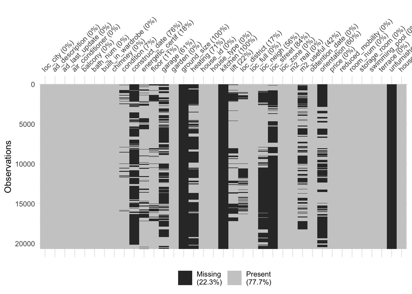
The data has many variables, but we are particularly interested in features such as construction year, district, number of rooms, lift and number of bathrooms, etc. to regress on our response price per square meter.
Let’s first drop features which have no data to build our working data set.
Bilbao <- data %>%
  filter(loc_city == "Bilbao") %>%
  select(-c(loc_city, garage, ad_description, ad_last_update, ground_size, kitchen, unfurnished, house_per_city, house_id, floor, loc_zone, loc_street, loc_neigh, obtention_date, orientation, loc_full, m2_useful)) %>%
  mutate(price_m2 = price/m2_real) %>%
  mutate(loc_district = gsub("Distrito", "", loc_district)) %>%
  mutate(bath_num = as.numeric(bath_num)) %>%
  filter(price_m2 >= quantile(price_m2, probs = 0.001)) %>%
  filter(price_m2 <= quantile(price_m2, probs = 0.999)) %>%
  mutate(condition = case_when(condition == "segunda mano/buen estado" ~ "used_ok",
                               condition == "promoción de obra nueva" ~ "new",
                               condition == "segunda mano/para reformar" ~ "used_to_reno")) %>%
  mutate(heating_type = case_when(heating == "calefacción central" ~ "central",
                             heating == "calefacción central: gas" ~ "central",
                             heating == "calefacción central: gas propano/butano" ~ "central",
                             heating == "calefacción central: gasoil" ~ "central",
                             heating == "calefacción individual" ~ "individual",
                             heating == "calefacción individual: bomba de frío/calor" ~ "individual",
                             heating == "calefacción individual: eléctrica" ~ "individual",
                             heating == "calefacción individual: gas" ~ "individual",
                             heating == "calefacción individual: gas natural" ~ "individual",
                             heating == "calefacción individual: gas propano/butano" ~ "individual",
                             heating == "calefacción individual: gas propano/butano" ~ "individual",
                             heating == "no dispone de calefacción" ~ "no_heat"
                             )) %>%
  mutate(id = row_number()) %>%
  filter(id != 3239) %>%
  select(-c(id, m2_real, heating, price))

# Save File
save(Bilbao, file = here("Data", "Houses_Bilbao", "Bilbao.Rda"))
Summary Statistics
Bilbao %>%
  tabyl(loc_district) %>%
  ggplot(aes(x = "", y = percent, fill = loc_district)) +
           geom_bar(stat = "identity", width =1, color="white") +
           coord_polar("y" , start = 0) +
  scale_fill_tq() +
  theme_minimal() +
  ggtitle("Proportion of houses per district")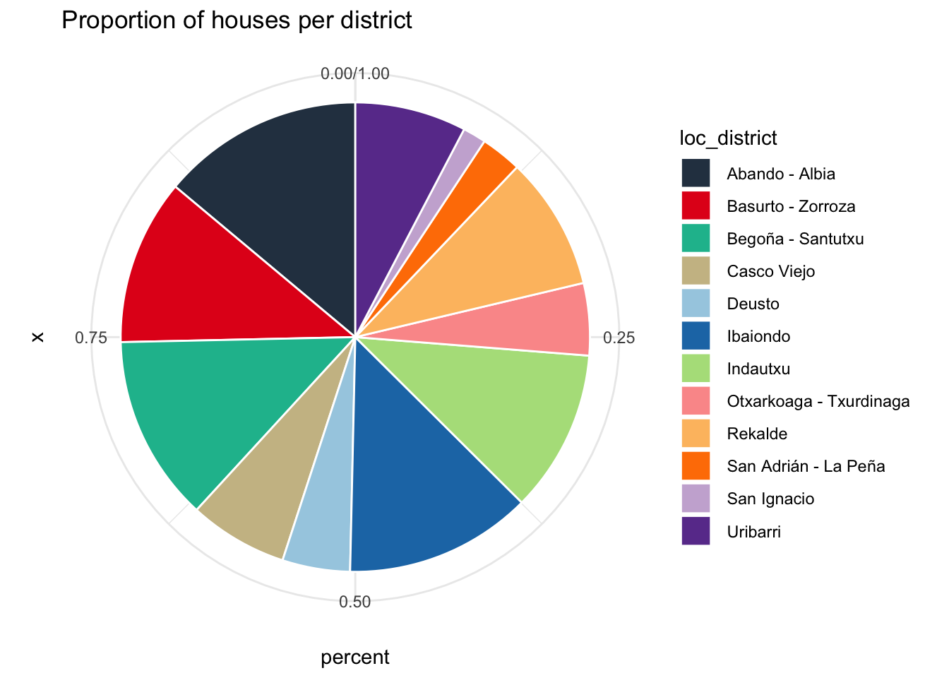
The graphic shows the proportion houses per district. In some cases two adjacent districts were grouped together in the data.
Square Meter Prices per District
Removing outliers <01 and >99 quantiles
Bilbao %>%
  group_by(loc_district) %>%
  summarise(Min = min(price_m2),
            Q25 = quantile(price_m2, probs = .25),
            Median = median(price_m2),
            Mean = mean(price_m2),
            Q75 = quantile(price_m2, probs = .75),
            Max = max(price_m2)) %>%
  arrange(desc(Median)) %>%
  dplyr::rename(District = loc_district) %>%
  kable(digits = 0, caption = "Statistic of price_m2 per district") %>%
kable_styling(full_width = T)| District | Min | Q25 | Median | Mean | Q75 | Max |
|---|---|---|---|---|---|---|
| Abando - Albia | 1882 | 3333 | 4444 | 4515 | 5294 | 8744 |
| Indautxu | 2333 | 3579 | 4091 | 4316 | 4778 | 8800 |
| Deusto | 249 | 2755 | 3184 | 3109 | 3569 | 4750 |
| Casco Viejo | 1478 | 2503 | 2963 | 3116 | 3667 | 5857 |
| Basurto - Zorroza | 314 | 1889 | 2835 | 2804 | 3531 | 6429 |
| Rekalde | 251 | 2224 | 2793 | 2765 | 3172 | 6042 |
| Begoña - Santutxu | 1024 | 2321 | 2757 | 2751 | 3133 | 5857 |
| San Ignacio | 1250 | 2288 | 2707 | 2797 | 3365 | 3931 |
| Uribarri | 45 | 2129 | 2517 | 2676 | 3110 | 8000 |
| Ibaiondo | 696 | 1963 | 2400 | 2543 | 3098 | 5556 |
| Otxarkoaga - Txurdinaga | 290 | 1791 | 2362 | 2385 | 2883 | 4982 |
| San Adrián - La Peña | 915 | 1797 | 2138 | 2223 | 2500 | 4808 |
It is better to visualize the table in a boxplot.
Bilbao %>%
  summarise(Min = min(price_m2),
            Q25 = quantile(price_m2, probs = .25),
            Median = median(price_m2),
            Mean = mean(price_m2),
            Q75 = quantile(price_m2, probs = .75),
            Max = max(price_m2)) %>%
  arrange(desc(Median))
Min Q25 Median Mean Q75 Max
1 45 2321.627 2962.963 3155.546 3750 8800Bilbao %>%
group_by(loc_district) %>%
ggplot(aes(x = loc_district, y = price_m2, fill = loc_district)) +
geom_boxplot() +
geom_hline(yintercept = 2962.963, linetype="dashed", color = "black") + # general Median
scale_fill_tq() +
theme_minimal() +
theme(axis.title.x=element_blank(),
axis.text.x=element_blank(),
axis.ticks.x=element_blank()) +
ggtitle("Boxplots of price_m2 per district") +
scale_y_continuous(labels = scales::dollar_format(prefix = "€"))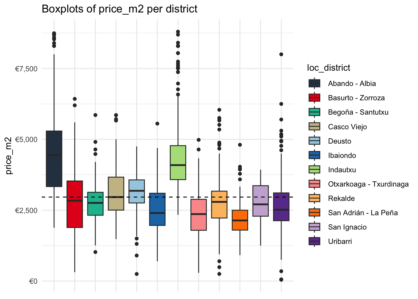
The districts Abando/Albia and Indautxu stand out for having particularly high square meter prices which are pushing the population median upwards. The differences between the other districts are comparabily not so high.
Let’s also have a look on the general distribution of price_m2
Bilbao %>%
  ggplot(aes(x = price_m2)) +
  geom_histogram(bins = 100) +
  ggtitle("House price/m2 in Euro") +
  scale_x_continuous(labels = scales::dollar_format(prefix = "€")) +
theme_minimal() 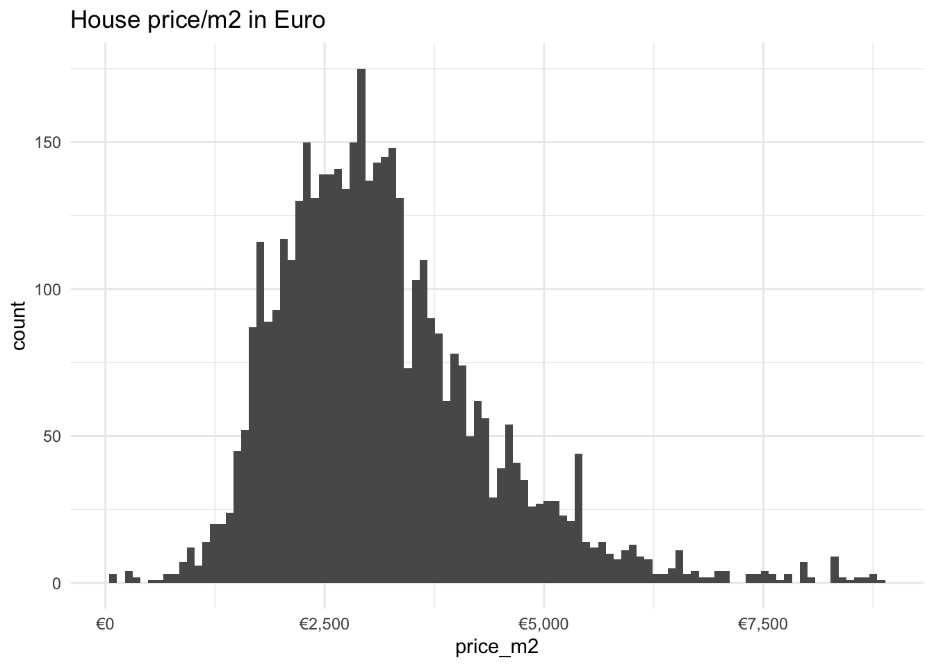
The distribution is relatively normal with a slight skewness to the right.
Overview of house features
Bilbao %>%
  filter(room_num <= 5) %>%
  tabyl(room_num, loc_district) %>%
  pivot_longer(
    cols = c(2:13),
    names_to = "loc_district",
    values_to = "Count"
  ) %>%
  group_by(loc_district) %>%
  mutate(Sum = sum(Count)) %>%
  mutate(Perc = Count/Sum * 100) %>%
  ggplot(aes(x = loc_district, y = Perc, fill = loc_district)) +
  geom_bar(position="dodge", stat = "identity") +
  facet_grid(cols = vars(room_num)) +
  scale_fill_tq() +
  theme_minimal() +
  theme(axis.title.x=element_blank(),
        axis.text.x=element_blank(),
        axis.ticks.x=element_blank()) +
  labs(title = "Percentage of Rooms per District")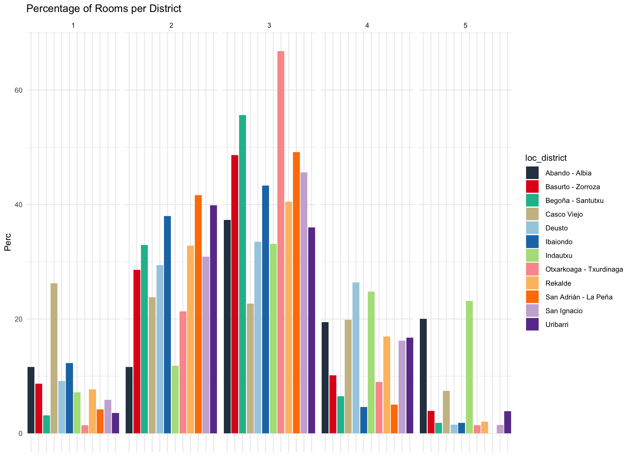
Most dwellings have 3 rooms. Interestingly Casco Viejo has a ove rproportionally many one room appartments while Indautxu and Abando have proportionally the largest number of 5 rooms.
Bilbao %>%
  ggplot(aes(x = heating_type, y = price_m2, fill = loc_district)) +
  geom_bar(position="dodge", stat = "identity") +
  scale_fill_tq() +
  theme_minimal() +
  labs(title = "Price_m2 per Heating Type") +
  scale_y_continuous(labels = scales::dollar_format(prefix = "€"))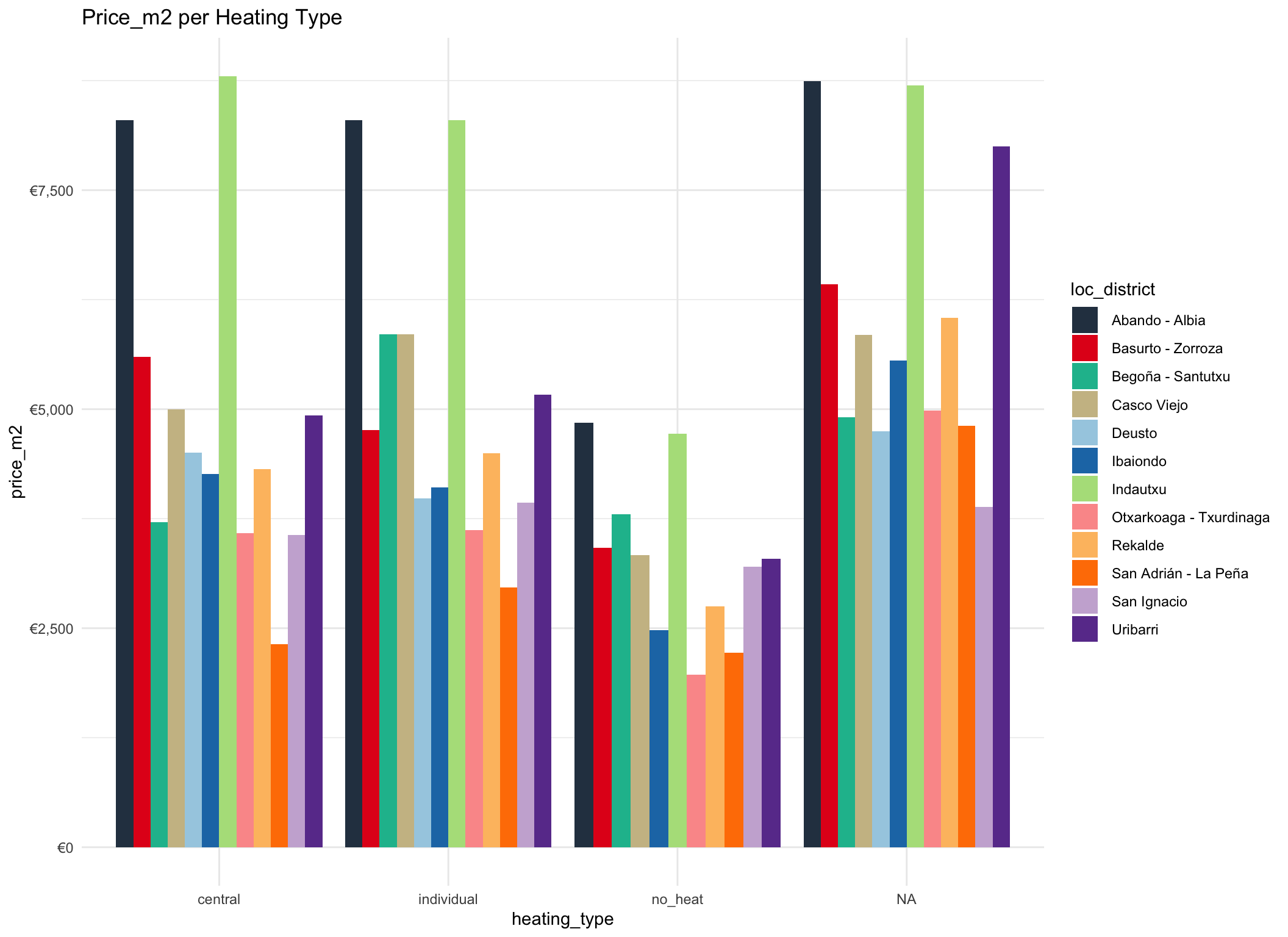
The type of heating doesn’t seem to affect very much.
Bilbao %>%
  tabyl(condition, loc_district) %>%
  pivot_longer(
    cols = c(2:13),
    names_to = "loc_district",
    values_to = "Count"
  ) %>%
  group_by(loc_district) %>%
  ggplot(aes(x = loc_district, y = Count, fill = loc_district)) +
  geom_bar(position="dodge", stat = "identity") +
  facet_grid(cols = vars(condition)) +
  scale_fill_tq() +
  theme_minimal() +
  theme(axis.title.x=element_blank(),
        axis.text.x=element_blank(),
        axis.ticks.x=element_blank()) +
  labs(title = "Absolute Count of House Condition per District")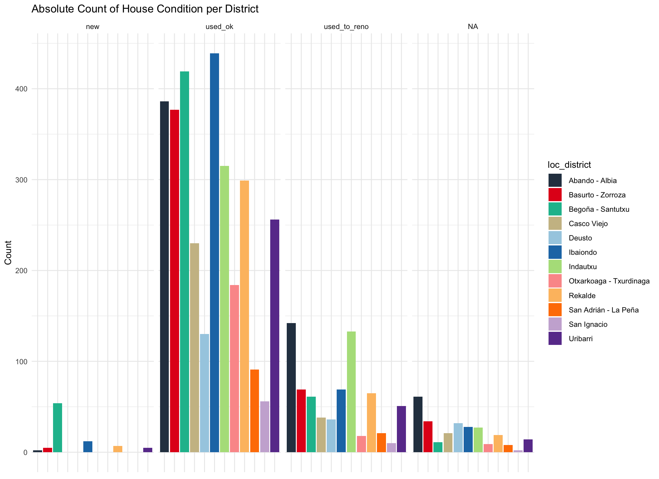
The majority of houses in the markets are second hand appartments in good condition.
Bilbao %>%
  ggplot(aes(x = condition, y = price_m2, fill = loc_district)) +
  geom_bar(position="dodge", stat = "identity") +
  scale_fill_tq() +
  theme_minimal() +
labs(title = "Price_m2 per Condition") 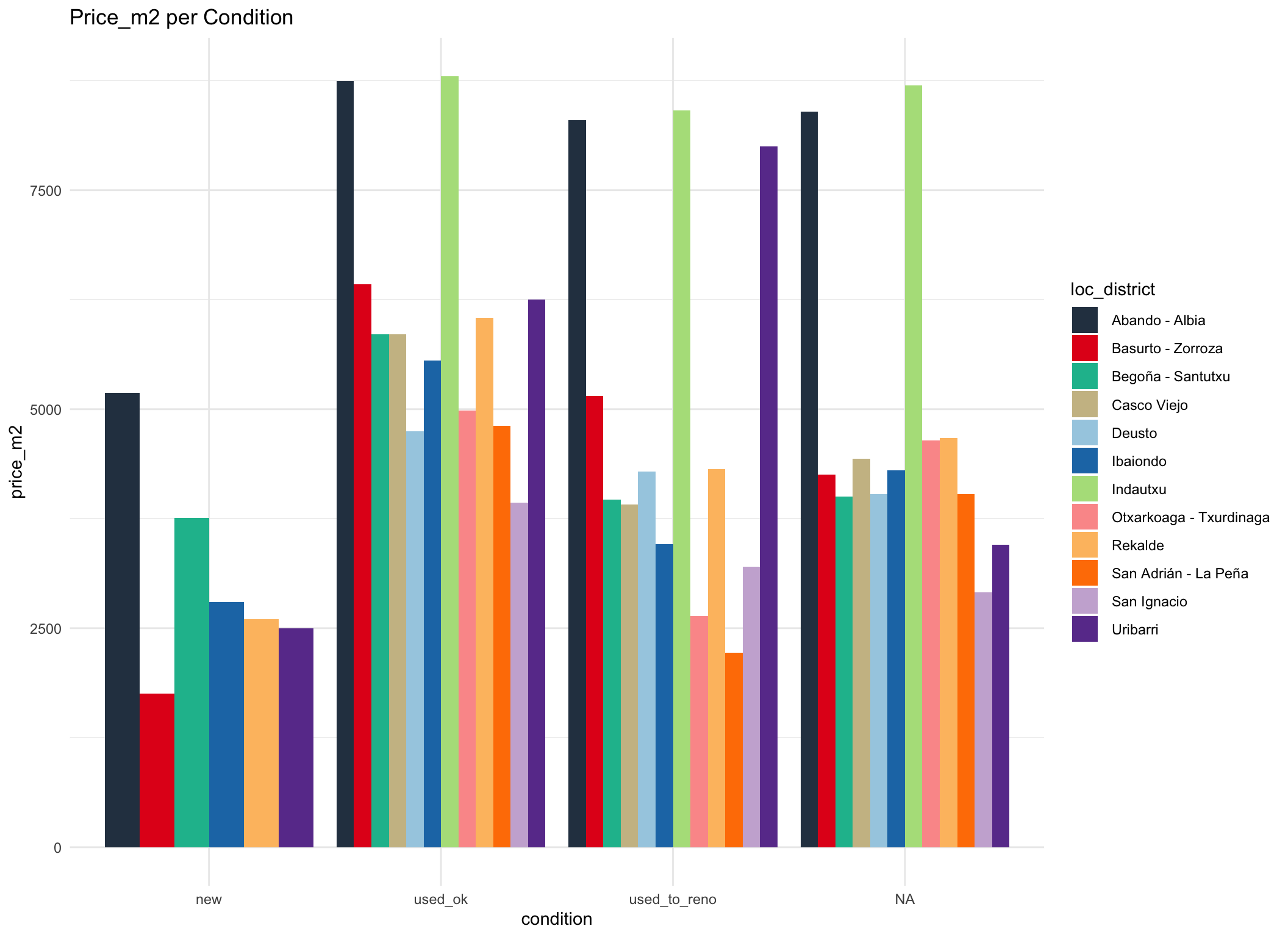
At first sight, it seems counter intuitive that new apartments cost less than second hand per sqare meter. Because of the hilliness of Bilbao, it might be that the new buildings are build in more peripheral areas of a district and therefore have a lower square meter price.
Construction Date
scatterplot(price_m2 ~ construct_date, data = Bilbao, grid = FALSE)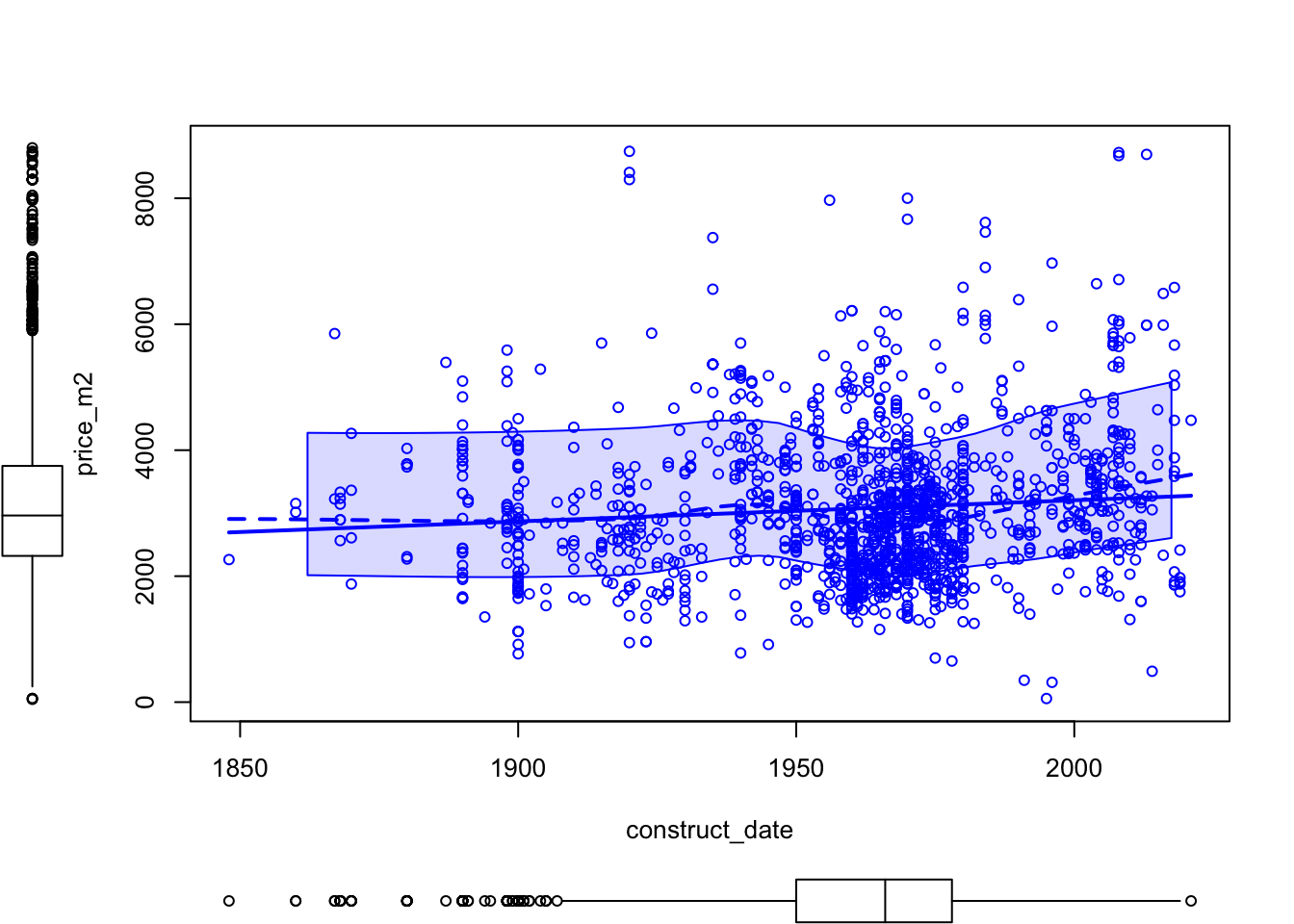
We see that there obvious relation between construction year and square meter price. Ad the same time we can observe that a great amount of houses were built during the period 1960-1975 corresponding to large migration from other Spanish provinces.
Development of Housing and Price
# Hiogh density region
Bilbao %>%
  ggplot(aes(x =construct_date, y = price_m2, fill = loc_district)) +
  geom_hdr(probs = c (0.9, 0.5)) +
  geom_point(shape = 21, size = 1.5) +
  scale_fill_tq() +
  theme_tq() +
  labs(title = "High density regions (Price_m2 ~ Date)") +
  facet_wrap(~ loc_district)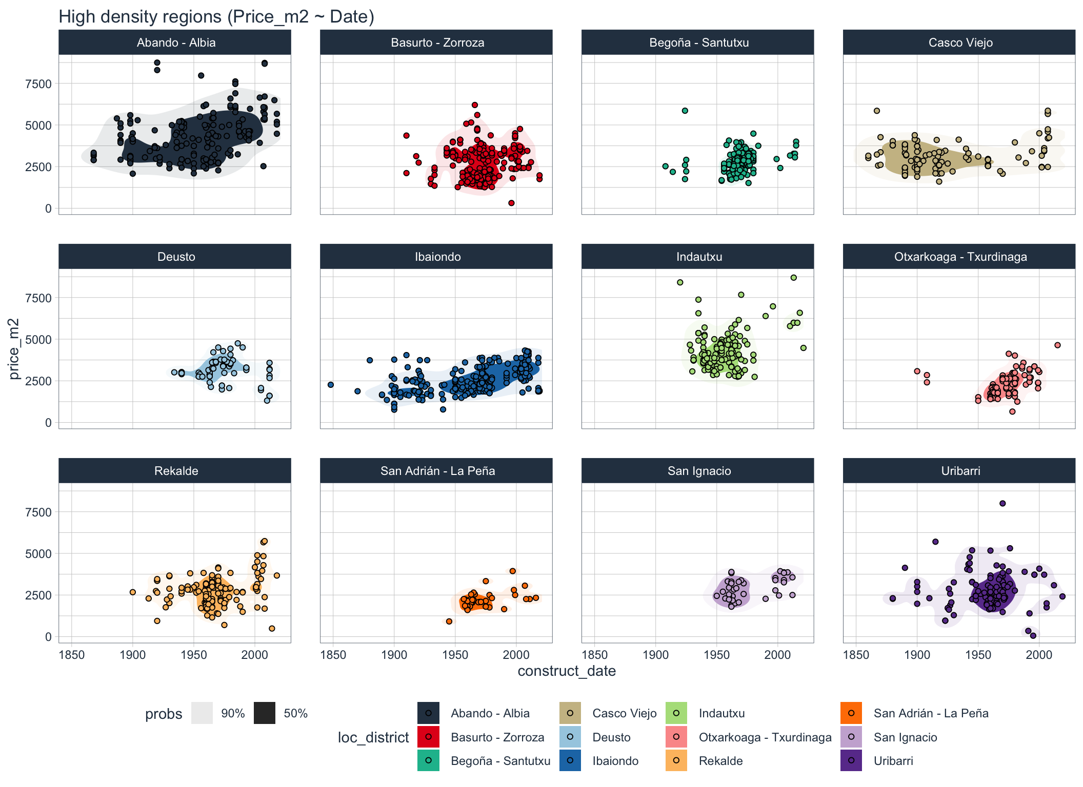
We can see that houses within district often share similar price ranges and construction years. Some older district live through a longer period of continuous construction, whereas in other construction seemed to had ben concentrated in smaller period.
Bilbao %>%
  filter(loc_district == " Abando - Albia" | loc_district == " San Ignacio" | loc_district == " Otxarkoaga - Txurdinaga") %>%
  ggplot(aes(x =construct_date, y = price_m2, fill = loc_district)) +
  geom_hdr(probs = c (0.9, 0.5)) +
  geom_point(shape = 21, size = 1.5) +
  scale_fill_tq() +
  theme_tq() +
  labs(title = "High density regions certain Neighborhoods")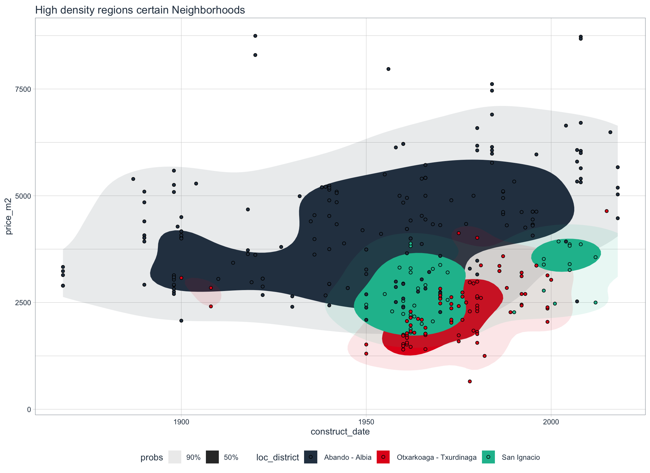
The clustering is specially visible for theese districts in a single graph.
Looking at Correlations
First, let us look at the correlations between all numeric features and response.
numeric = Bilbao %>%
  select(where(is.numeric))

ggcorr(numeric, label = TRUE, label_size = 2, label_color = "white") +
  scale_fill_paletteer_c("viridis::plasma") +
  labs(title = "Correlations (Numeric Variables)")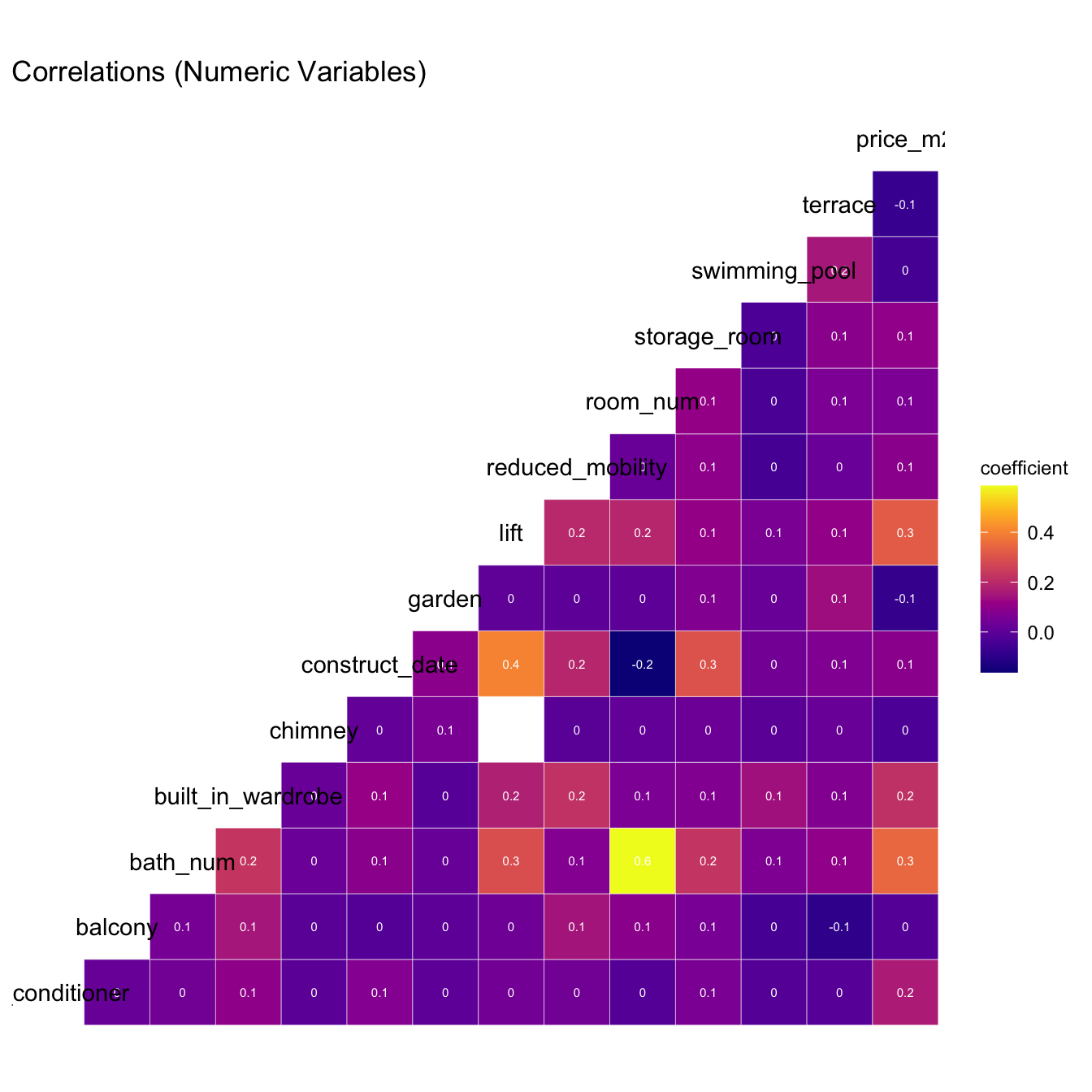
Especially important are the correlations with response variable.
Bilbao %>%
  corr_var(price_m2)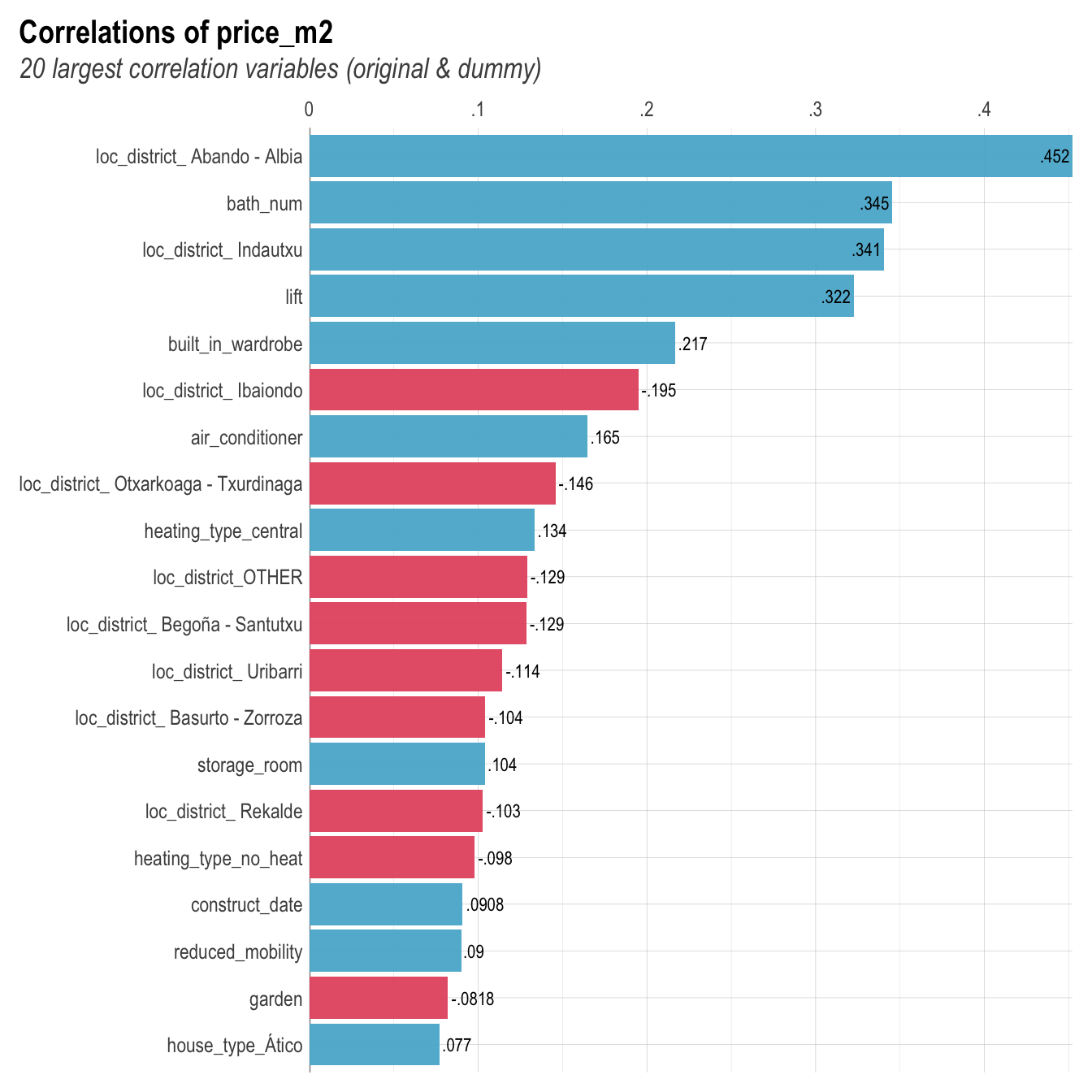
Using the simple correlation we can see that being loacted in the district of Abando/Albia has the highest positive correlation with the square meter price.
Modeling
Now, since we got an overview of the data, we can start to analyzenthe relationships between the features and the response more in depth.
Splitting the Data
First we split the data into a train and test set where 3/4 of the whole data is reserved for training and the rest for testing. We also use strata = "price_m2" to make sure that the distribution of price_m2 is equal between training and testing set.
set.seed(123)
split <- initial_split(Bilbao, prop = 0.75,
                       strata = "price_m2")
data_train  <- training(split)
data_test   <- testing(split)
Missing Data
There is missing data. Because some models (like OLS) cannot handle NAs we will interpolate these using a KNN Algorithm.
vis_miss(Bilbao, cluster = TRUE)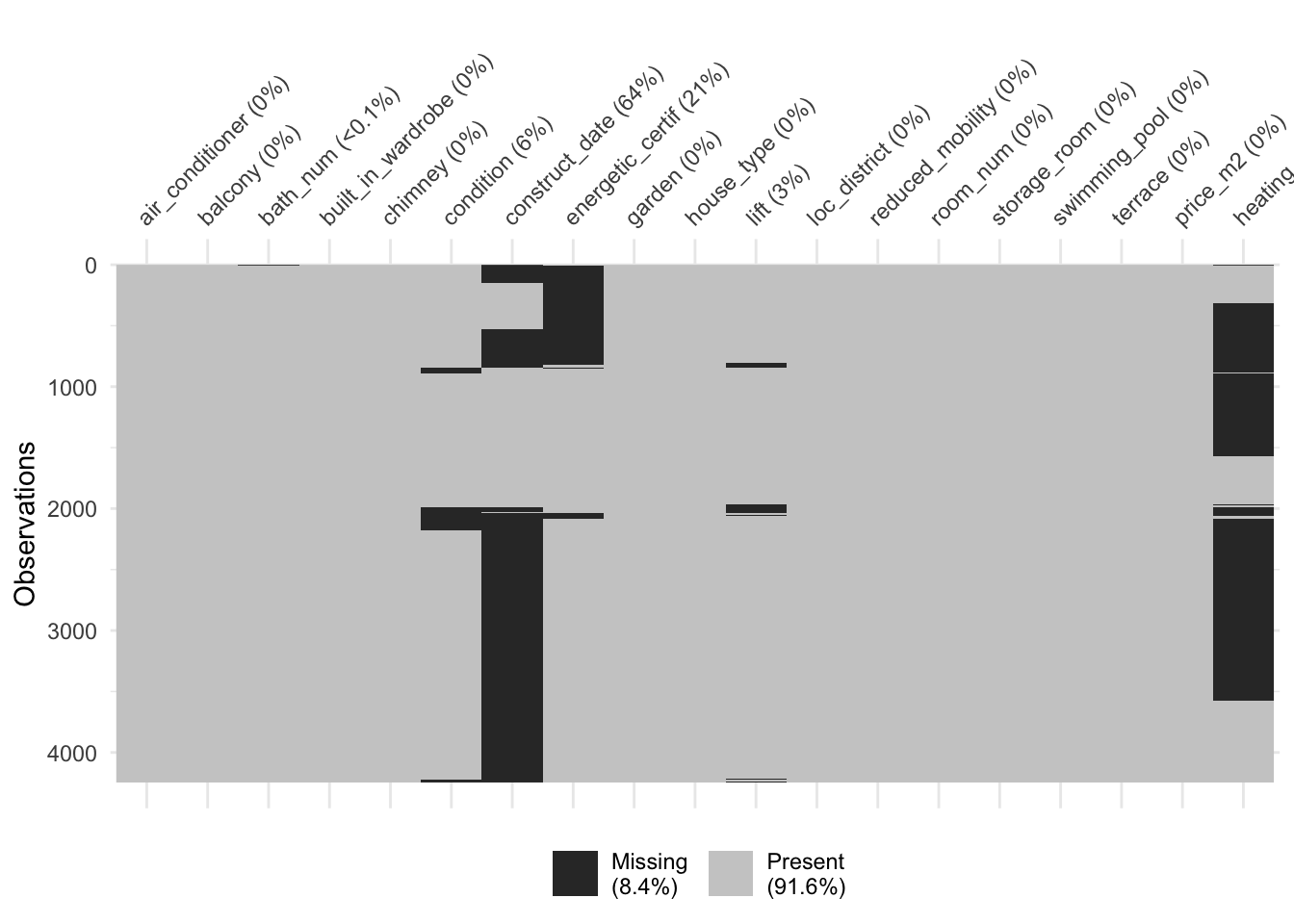
Create a Recipe
The function recipe() allows to preprocess the data before modeling. It can be applied to training and testing data. The advantage of uf using recipe() is that it avoids data leakage between data sets. Data leakage occurs when data transformation steps are processed on the entire data set before it is subdivided into training and testing splits. E.g., if a min-max transformation would be applied on the whole data set before splitting, the individual splits would be biased towards to global minimum and maximum. In a resampling and cross validation context, recipe() ensures that the data preprocessing is conducted after every iteration of data splitting.
model_rec <- recipe(
  price_m2 ~ .,
  data= data_train) %>%
  step_zv(all_predictors()) %>%
  step_dummy(all_nominal()) %>%
  step_impute_knn(all_predictors(), neighbors = 10) %>%
  prep(training = data_train, retain=TRUE, verbose=TRUE)
oper 1 step zv [training]
oper 2 step dummy [training]
oper 3 step impute knn [training]
The retained training set is ~ 0.97 Mb in memory.trainSet.prep <- bake(model_rec, new_data = data_train, composition='matrix')
trainSet = as.data.frame((trainSet.prep))
testSet.prep<-bake(model_rec, new_data = data_test, composition='matrix')
testSet = as.data.frame((testSet.prep))Experimenting with various Models
Let’s first have a look at how well different models perform on the data. For the resampling method we perform a 10-fold cross validation repeated 5 times.
Initialize Models
myControl = trainControl(method = 'cv',
                         number = 10,
                         repeats = 5,
                         verboseIter = FALSE,
                         savePredictions = TRUE,
                         allowParallel = T)


parallel_start(6)

set.seed(174)
Linear.Model = train(price_m2 ~.,
                     data = trainSet,
                     metric = 'RMSE',
                     method = 'lm',
                     preProcess = c('center', 'scale'),
                     trControl = myControl)


set.seed(174)
Glmnet.Model = train(price_m2 ~ .,
                     data = trainSet ,
                     metric = 'RMSE',
                     method = 'glmnet',
                     preProcess = c('center', 'scale'),
                     trControl = myControl)


set.seed(174)
Rapid.Ranger = train(price_m2 ~ .,
                     data = trainSet,
                     metric = 'RMSE',
                     method = 'ranger',
                     preProcess = c('center', 'scale'),
                     trControl = myControl)


set.seed(174)
Basic.Knn <- train(price_m2 ~ .,
             method     = "knn",
             tuneGrid   = expand.grid(k =1:3),
             trControl  = myControl,
             metric= "RMSE",
             data = trainSet)


set.seed(174)
Xgb.Super <- train(price_m2~.,
                   method = "xgbTree",
                   tuneLength = 4,
                   trControl = myControl,
                   metric= "RMSE",
                   data = trainSet)

parallel_stop()
suite.of.models = list("LINEAR.MODEL" = Linear.Model,
"GLMNET.MODEL" = Glmnet.Model,
"RANGER.QUEST" = Rapid.Ranger,
"KNN.SIMPLE" = Basic.Knn,
"XGB.SUPER"= Xgb.Super)
resamps = resamples(suite.of.models)
dotplot(resamps, metric = 'RMSE')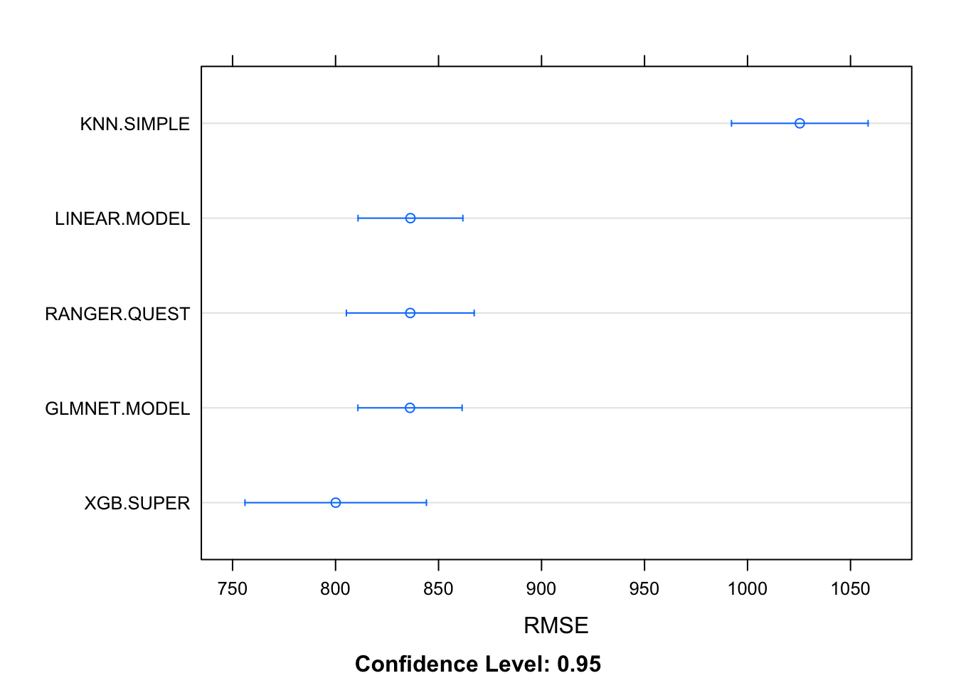
XGBoost perfomes best on the training data. Let’s test it on the test data.
TESTING MODELS ON TEST SET
Evaluate.Prediction <- function(model, model.label, testData, ytest, grid = NULL) {

  #capture prediction time
  ptm <- proc.time()
  # use test data to make predictions
  pred <- predict(model, testData)
  tm <- proc.time() - ptm

  Pred.metric<- postResample(pred = pred, obs = ytest)
  RMSE.test <- c(Pred.metric[[1]])
  RSquared.test <- c(Pred.metric[[2]])
  MAE.test <- c(Pred.metric[[3]])


  Summarised.results = NULL
  if (is.null(grid)) {
    Summarised.results = data.frame(predictor = c(model.label) ,  RMSE = RMSE.test , RSquared = RSquared.test, MAE = MAE.test, time = c(tm[[3]]))
  } else {
    .grid = data.frame(predictor = c(model.label) , RMSE = RMSE.test , RSquared = RSquared.test, MAE = MAE.test, time = c(tm[[3]]))
    Summarised.results = rbind(grid, .grid)}


  Summarised.results }


METRIC.GRID <- Evaluate.Prediction (Rapid.Ranger, "RAPID.QUEST", testSet, testSet$price_m2, grid=NULL)

METRIC.GRID <- Evaluate.Prediction (Glmnet.Model, "GLMNET.MODEL", testSet, testSet$price_m2, grid=METRIC.GRID)

METRIC.GRID <- Evaluate.Prediction (Basic.Knn, "KNN.SIMPLE", testSet, testSet$price_m2, grid=METRIC.GRID)

METRIC.GRID <- Evaluate.Prediction (Linear.Model, "LINEAR.MODEL", testSet, testSet$price_m2, grid=METRIC.GRID)

METRIC.GRID <- Evaluate.Prediction (Xgb.Super, "XGB.SUPER", testSet, testSet$price_m2, grid=METRIC.GRID)


kable(METRIC.GRID[order(METRIC.GRID$RMSE, decreasing=F),]) %>%
kable_styling(bootstrap_options = c("striped", "hover", "condensed"))| predictor | RMSE | RSquared | MAE | time | |
|---|---|---|---|---|---|
| 5 | XGB.SUPER | 773.6237 | 0.6066140 | 576.2671 | 0.035 |
| 1 | RAPID.QUEST | 805.4272 | 0.5733575 | 584.3447 | 0.032 |
| 2 | GLMNET.MODEL | 822.0240 | 0.5559522 | 607.2007 | 0.013 |
| 4 | LINEAR.MODEL | 822.3261 | 0.5553493 | 607.3631 | 0.006 |
| 3 | KNN.SIMPLE | 1023.4154 | 0.3434201 | 720.6059 | 0.063 |
Also here, XGBoost has the smallest RMSE and highest R2. Let’s tune this model for further examination.
XGBoost Modelling
Preprocessing
First we start again by dividing the data into training and testing samples. Again, we use price_m2 as a strata to ensure that the distribution of the response is eqaul between the testing and training sets. Then we create a recipe.
set.seed(123)
split <- initial_split(Bilbao, prop = 0.75,
                       strata = "price_m2")
data_train  <- training(split)
data_test   <- testing(split)

XGB_rec <- recipe(
  price_m2 ~ .,
  data= data_train) %>%
  step_zv(all_predictors()) %>%
  step_dummy(all_nominal()) %>%
  step_impute_knn(all_predictors(), neighbors = 10) %>%
  prep()
Apply pre-processing to randomly divide train data in subsets.
set.seed(123)
cv_folds <-recipes::bake(
    XGB_rec,
    new_data = data_train)%>%
  rsample::vfold_cv(v = 5)

train.ready<-juice(XGB_rec)
test.ready<-bake(XGB_rec, new_data = data_test)
Modelling specifications
Define XGBoost modelling specifications and hyper parameters for tuning.
Model.XGB <-
  boost_tree(
    mode = "regression",
    trees = 1000,
    min_n = tune(),
    tree_depth = tune(),
    learn_rate = tune(),
    loss_reduction = tune()) %>%
  set_engine("xgboost", objective = "reg:squarederror")
Specify the model parameters
# grid specification
XGB.aspects <-
  dials::parameters(
    min_n(),
    tree_depth(),
    learn_rate(),
    loss_reduction())
Grid Space
Set up a grid space which covers the hyper parameters XGB.aspects.
xgboost_grid <-
dials::grid_max_entropy(
XGB.aspects, size = 200)
kable(head(xgboost_grid))| min_n | tree_depth | learn_rate | loss_reduction |
|---|---|---|---|
| 19 | 4 | 0.0000000 | 0.0024421 |
| 15 | 11 | 0.0502801 | 0.0000204 |
| 38 | 3 | 0.0000000 | 0.0000000 |
| 7 | 10 | 0.0000001 | 0.0002759 |
| 38 | 8 | 0.0000000 | 0.0000001 |
| 37 | 5 | 0.0287556 | 0.0000003 |
Create a workflow
xgboost_wf <-
workflows::workflow() %>%
add_model(Model.XGB) %>%
add_formula(price_m2 ~ .)
Hyper parameter searching
In this step R searches for the optimal hyper parameters by iteratively applying the different hyper parameters to multiple training samples. This step can take a while to compute.
'parallel_start(6)

TUNE.XGB <- tune::tune_grid(
  object = xgboost_wf,
  resamples = cv_folds,
  grid = xgboost_grid,
  metrics = yardstick::metric_set(yardstick::rmse, yardstick::rsq, yardstick::rsq_trad, yardstick::mae),
  control = tune::control_grid(verbose = FALSE))

parallel_stop()

saveRDS(TUNE.XGB, file = here("Data", "Tune_XGB.RData"))'
Finalize optimal tune
Extract parameters with lowest RMSE.
TUNE.XGB <- readRDS(here("Data", "Houses_Bilbao","Tune_XGB.RData"))

param_final <- TUNE.XGB %>%select_best(metric = "rmse")
Finalize XGBoost with optimal tune.
xgboost_wf2 <- xgboost_wf%>%
finalize_workflow(param_final)
Fit the final model
Fit final model on the preprocessed training data.
XGB.model <- xgboost_wf2 %>%
fit(train.ready)
Extract important features.
XGB.model %>%
  pull_workflow_fit() %>%
  vip()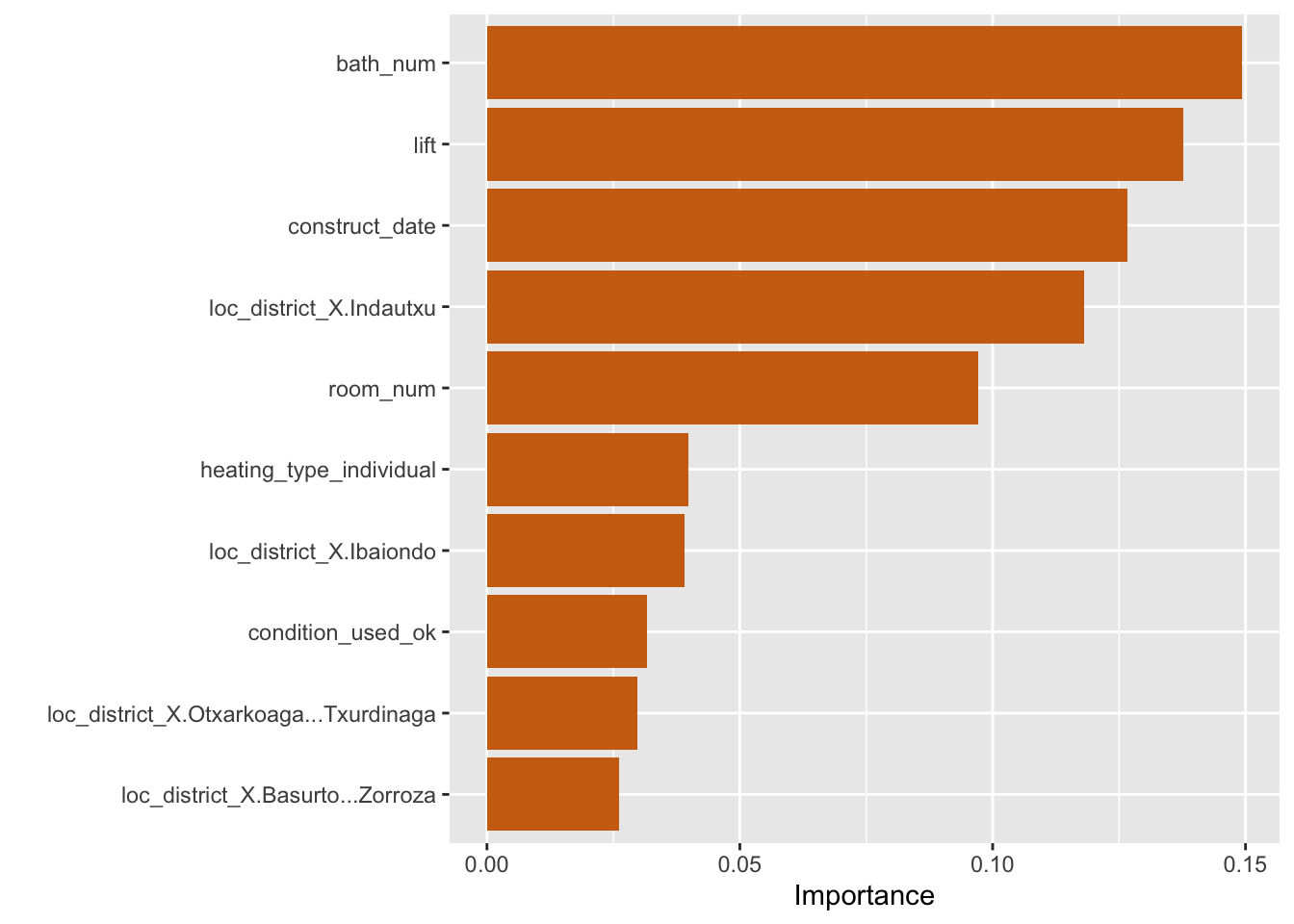
The number of bathrooms, whether the appartment has a lift and the construction date seems to be the most important determinants for the square meter price.
Predict on Test set.
Let’s evaluate the XGBoost model on the test data by computing the RMSE.
# use the training model fit to predict the test data
XGB_res <- predict(XGB.model, new_data = test.ready %>% select(-price_m2))

XGB_res <- bind_cols(XGB_res, test.ready %>% select(price_m2))

XGB_metrics <- metric_set(yardstick::rmse, yardstick:: mae)

kable(XGB_metrics(XGB_res, truth = price_m2, estimate = .pred))| .metric | .estimator | .estimate |
|---|---|---|
| rmse | standard | 799.5876 |
| mae | standard | 590.3934 |
We can asses the fit of the pridiction by plotting them against the actual observations from the testing samples. We can see that the model works good up to 5000 Euro per square meter. For higher the model tends to underestimate the real prices.
ggplot(XGB_res, aes(x = price_m2, y = .pred)) +
    # Create a diagonal line:
    geom_abline(lty = 2) +
    geom_point(alpha = 0.5) +
    labs(y = "Predicted Sale Price", x = "SalePrice") +
    # Scale and size the x- and y-axis uniformly:
    coord_obs_pred() +
  theme_minimal()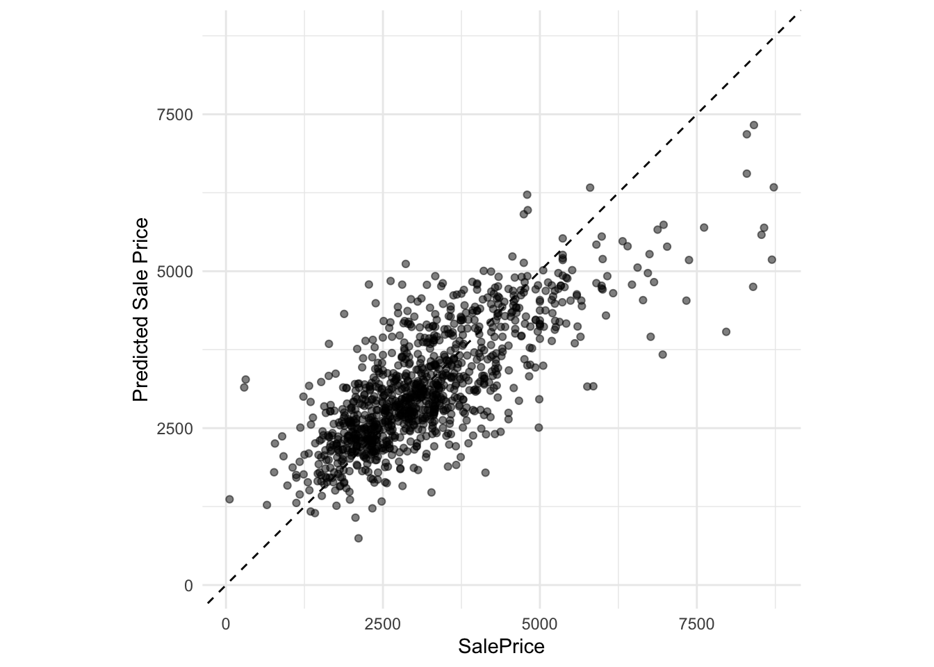
Explainer
Finaly, we can explore the model prediction using the Explainer from modelstudio() which supplies metrics on feature importance, drop dow charts and Shapley values.
explainer<- explain_tidymodels(model = XGB.model,
                    data = test.ready,
                    y = test.ready$price_m2,
                    label = "XGBoost")
Preparation of a new explainer is initiated
-> model label : XGBoost
-> data : 1063 rows 39 cols
-> data : tibble converted into a data.frame
-> target variable : 1063 values
-> predict function : yhat.workflow will be used ( default )
-> predicted values : No value for predict function target column. ( default )
-> model_info : package tidymodels , ver. 1.0.0 , task regression ( default )
-> predicted values : numerical, min = 744.7933 , mean = 3149.823 , max = 7328.426
-> residual function : difference between y and yhat ( default )
-> residuals : numerical, min = -2960.2 , mean = 17.77691 , max = 3933.913
A new explainer has been created! modelStudio(explainer)